Plot Data with Charts

In this tutorial, you will learn how to use pipelines to plot data as charts.

The Tenzir Query Language (TQL) excels at slicing and dicing even the most complex shapes of data. But turning tabular results into actionable insights often calls for visualization. This is where charts come into play.

Available chart types

Tenzir supports four types of charts, each with a dedicated operator:

1. Pie: chart_pie
2. Bar: chart_bar
3. Line: chart_line
4. Area: chart_area

How to plot data

Plotting data in the Explorer involves three steps:

1. Run a pipeline to prepare the data.
2. Add a chart_* operator to render the plot.
3. View the chart below the Editor.

After generating a chart, you can download it or add it to a dashboard to make it permanent refresh it periodically.

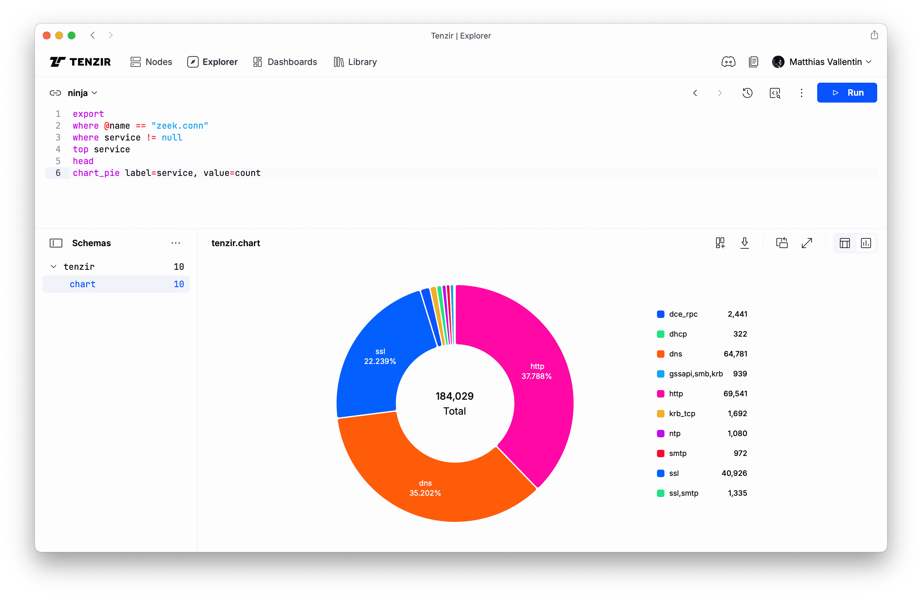
Example: Here's how you generate a pie chart that shows the application breakdown from Zeek connection logs:

export
where @name == "zeek.conn"
where service != null
top service
head
chart_pie label=service, value=count

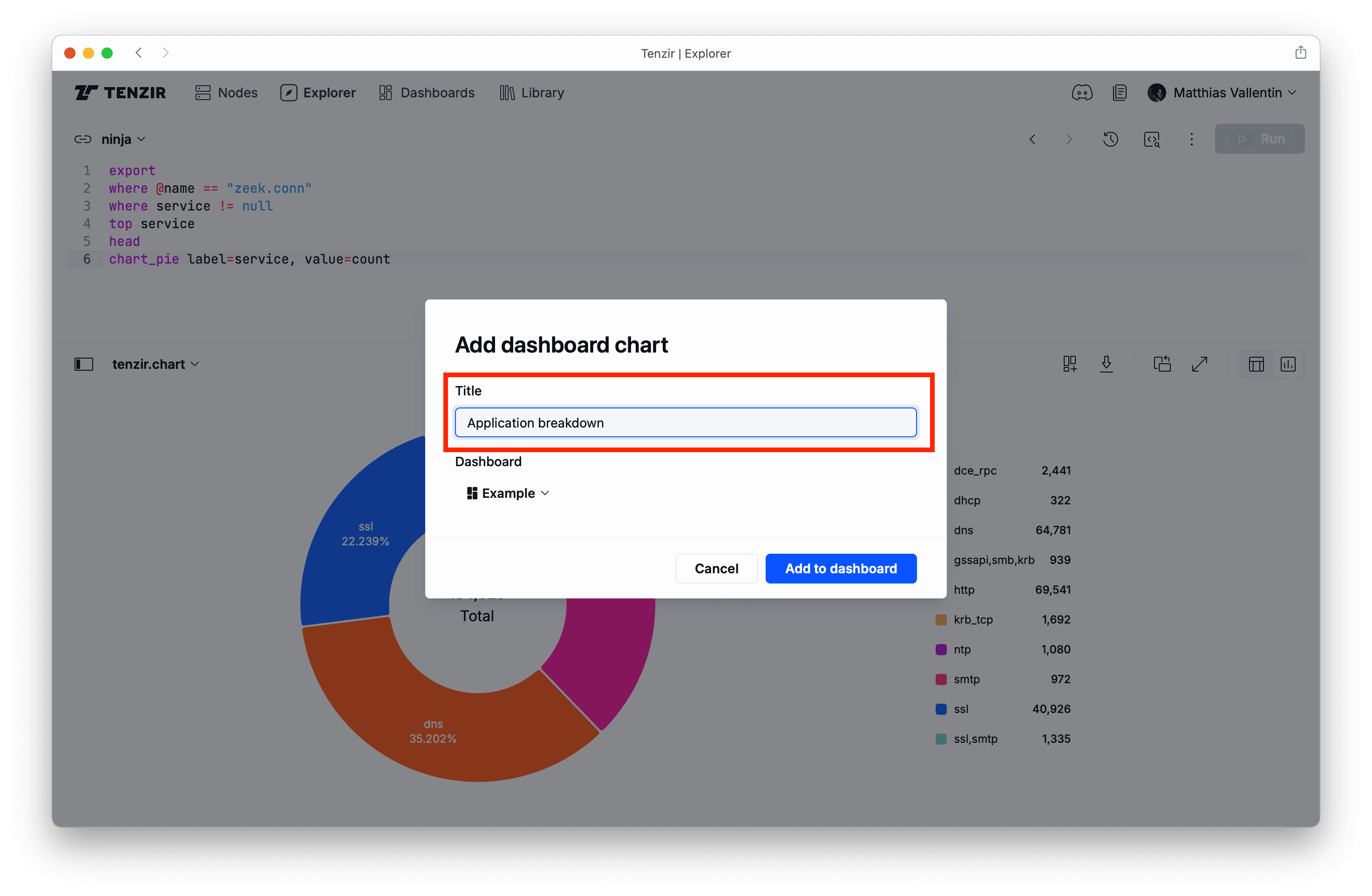
Add a chart to a dashboard

To make a chart permanent:

1. Click the Dashboard button.

   

2. Enter a title for the chart, then click Add to Dashboard.

   

3. View the chart in your dashboard.

   

🎉 Congratulations! Your chart is now saved and will automatically reload when you open the dashboard.

Download a chart

Download a chart in the Explorer as follows:

1. Click the download button in the top-right corner.

   

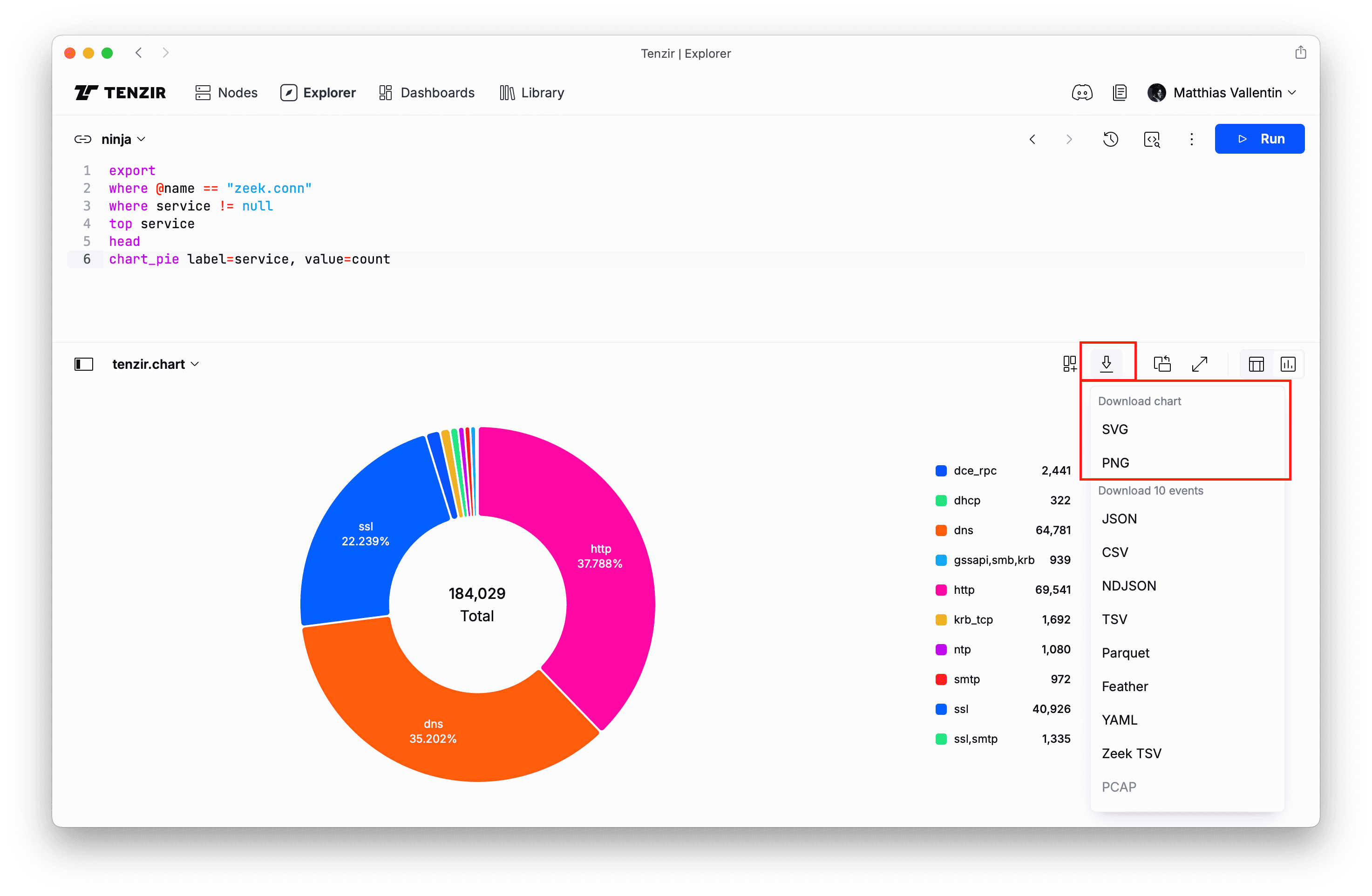
2. Choose PNG or SVG to save the chart as an image.

You can also download a chart on a dashboard:

1. Click the three-dot menu in the top-right corner of the chart.

2. Click Download

   

3. Choose PNG or SVG to save the chart as an image.

⬇️ You have now successfully save the chart to your computer. Enjoy.

Master essential charting techniques

Now that you know how to create charts, let us explore some common techniques to enhance your charting skills.

Plot counters as bar chart

A good use case for bar charts is visualization of counters of categorical values, because comparing bar heights is an effective way to gain a relative understanding of the data at hand.

1. Shape your data: Suppose you want to create a bar chart showing the outcomes of coin flips. First, generate a few observations:

   from {}
   repeat 20
   set outcome = "heads" if random().round() == 1 else "tails"
   summarize outcome, n=count()

   Sample output:

   {outcome: "tails", n: 9}
   {outcome: "heads", n: 11}

2. Plot the data: Add the chart_bar operator to visualize the counts.

   Map the outcome and count fields to the x-axis and y-axis:

   from {outcome: "tails", n: 9},
        {outcome: "heads", n: 11}
   chart_bar x=outcome, y=n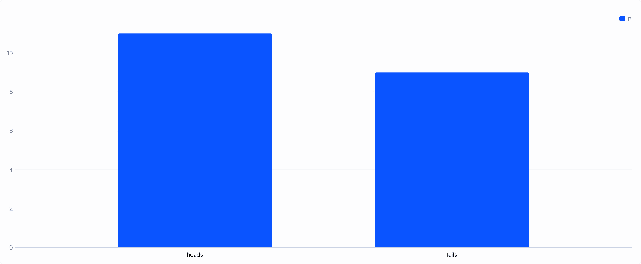

   

Group and stack bars

Sometimes, your data has a third dimension. You can group multiple series into a single plot.

Example with a time dimension:

from (
  {outcome: "tails", n: 9, time: "Morning"},
  {outcome: "heads", n: 11, time: "Morning"},
  {outcome: "tails", n: 14, time: "Afternoon"},
  {outcome: "heads", n: 15, time: "Afternoon"},
  {outcome: "tails", n: 4, time: "Evening"},
  {outcome: "heads", n: 12, time: "Evening"},
)
chart_bar x=outcome, y=n, group=time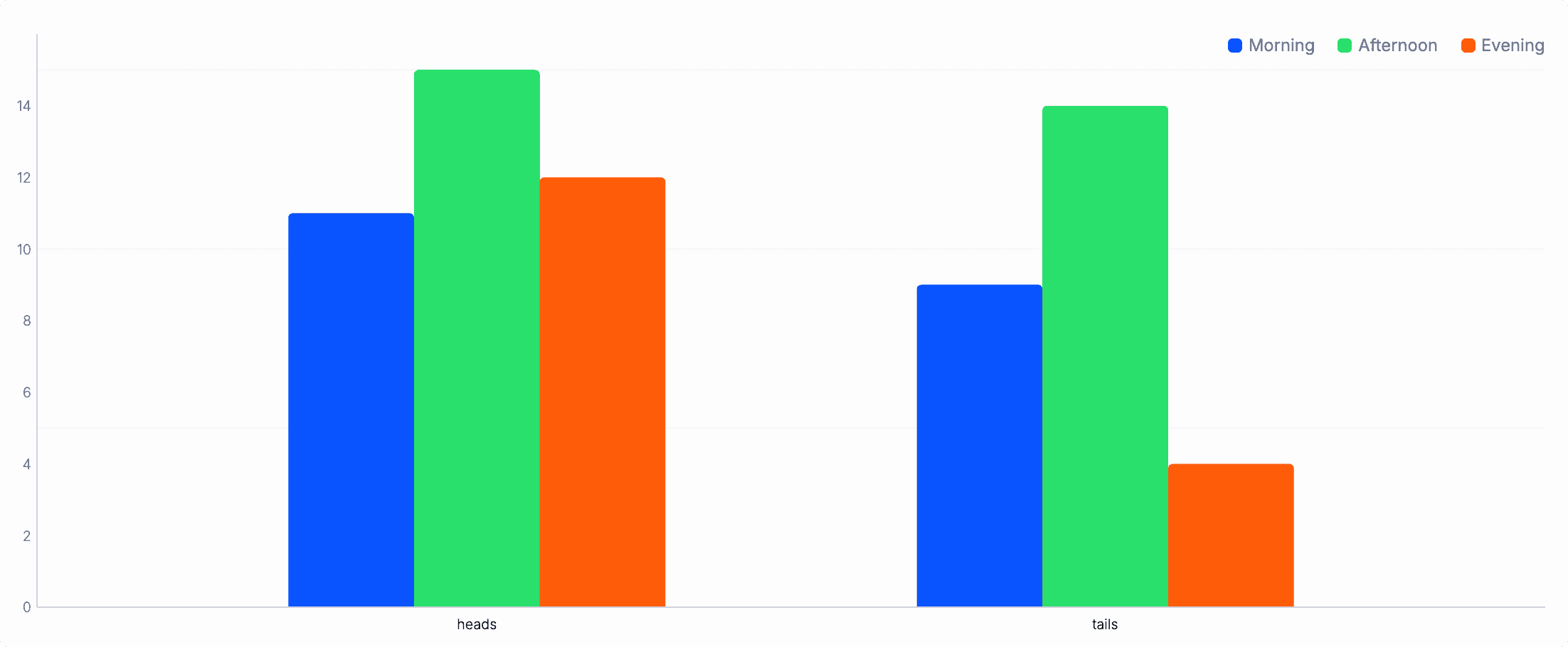

To stack the grouped bars, add position="stacked":

from (
  {outcome: "tails", n: 9, time: "Morning"},
  {outcome: "heads", n: 11, time: "Morning"},
  {outcome: "tails", n: 14, time: "Afternoon"},
  {outcome: "heads", n: 15, time: "Afternoon"},
  {outcome: "tails", n: 4, time: "Evening"},
  {outcome: "heads", n: 12, time: "Evening"},
)
chart_bar x=outcome, y=n, group=time, position="stacked"

Scale the y-axis logarithmically

If your data spans several orders of magnitude, log scaling can make smaller values visible.

Example without log scaling:

from (
  {outcome: "A", n: 3},
  {outcome: "B", n: 5},
  {outcome: "C", n: 10},
  {outcome: "D", n: 21},
  {outcome: "E", n: 10000},
)
chart_bar x=outcome, y=n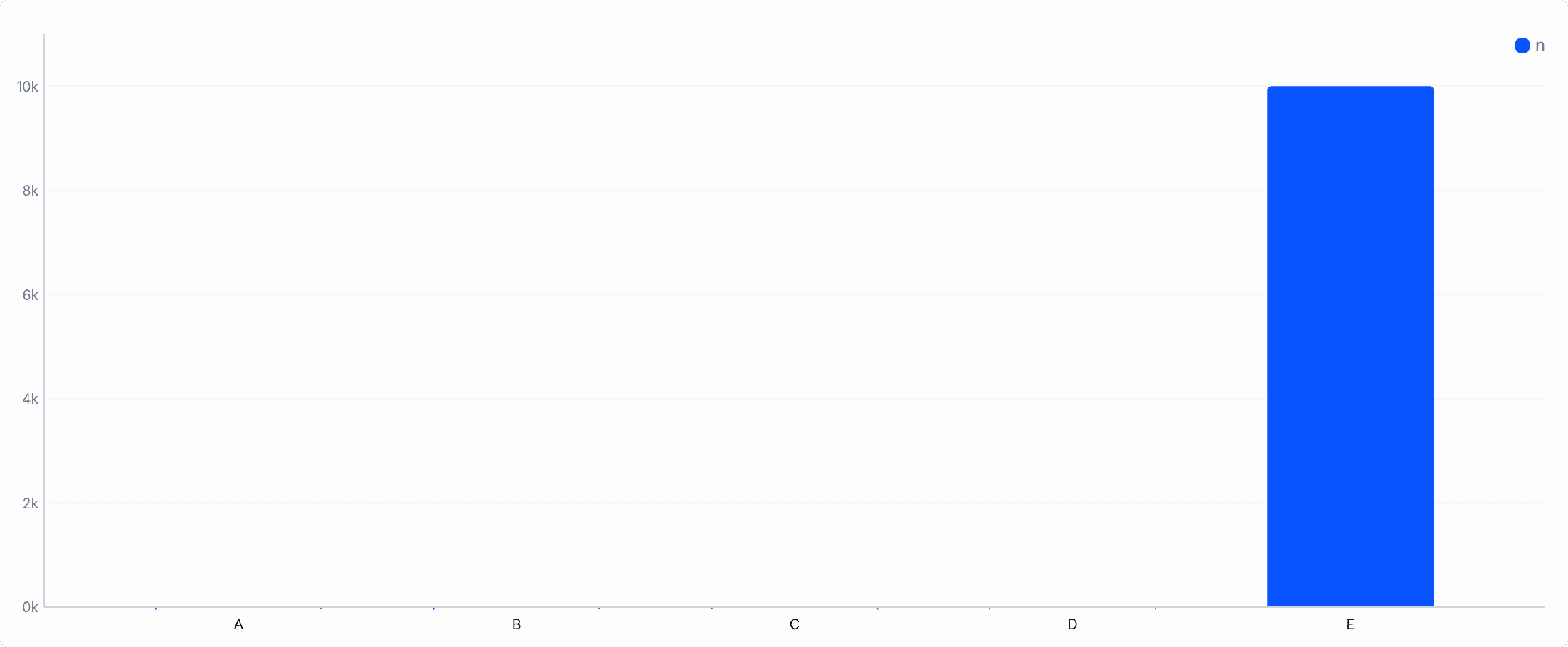

The large value (E) dominates the chart, hiding the smaller categories.

Enable log scaling via y_log=true to reveal them:

from (
  {outcome: "A", n: 3},
  {outcome: "B", n: 5},
  {outcome: "C", n: 10},
  {outcome: "D", n: 21},
  {outcome: "E", n: 10000},
)
chart_bar x=outcome, y=n, y_log=true

Now, you can clearly see all the values! 👀

Interpreting Log-Scaled Plots

Log scaling removes linearity. Comparing bar heights no longer reflects a simple numeric ratio. Stacked values are not additive anymore.

Plot compositions as pie chart

Pie charts are well-understood and frequently occur in management dashboards. Let's plot some synthetic data with the chart_pie operator:

from (
  {category: "A", percentage: 40},
  {category: "B", percentage: 25},
  {category: "C", percentage: 20},
  {category: "D", percentage: 10},
  {category: "E", percentage: 5},
)
chart_pie label=category, value=percentage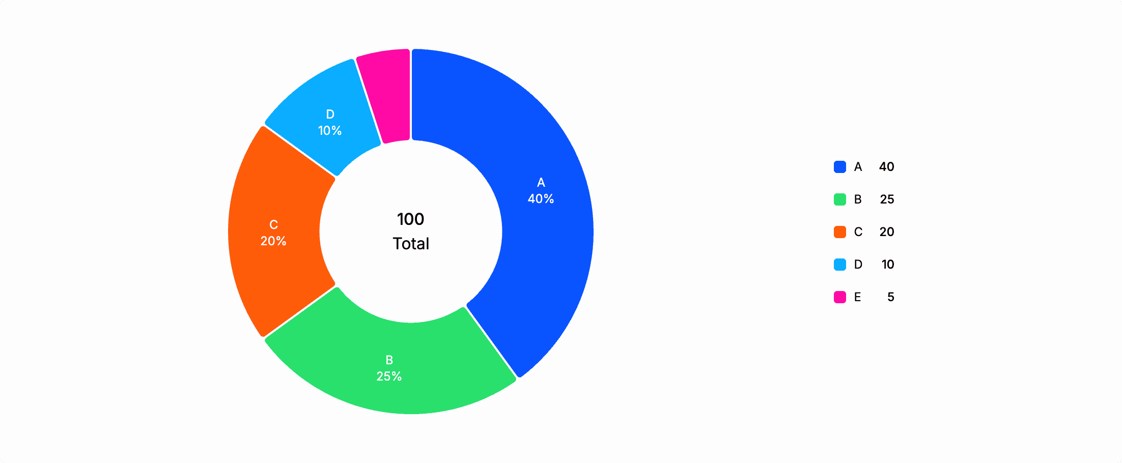

To provide a consistent user experience across all chart types, chart_pie treats label and x as interchangeable, as well as value and y. This mapping makes intuitive sense when you consider a pie chart as a bar chart rendered in a radial coordinate system.

Bar Charts > Pie Charts

Use bar charts when you can and pie charts when you must. Why? Pie charts are often considered inferior to bar charts because they rely on human perception of angles, which is less accurate than judging lengths, making comparisons between categories harder. Bar charts allow for quick, precise comparisons, handle many categories cleanly, and often do not require labels, while pie charts become cluttered and confusing with numerous slices. Bar charts also allow easy sorting, are more space-efficient, and tend to stay cleaner without unnecessary visual distractions like 3D effects. Overall, bar charts communicate data more clearly, accurately, and efficiently than pie charts.

Plot metrics as line chart

Line charts come in handy when visualizing data trends over a continuous scale, such as time series data.

1. Shape your data: For our line chart demo, we'll use some internal node metrics provided by the metrics operator. Let's look at the RAM usage of the node:

   metrics "process"
   drop swap_space, open_fds
   head 3

   {timestamp: 2025-04-27T18:16:17.692Z, current_memory_usage: 2363461632, peak_memory_usage: 4021136}
   {timestamp: 2025-04-27T18:16:18.693Z, current_memory_usage: 2366595072, peak_memory_usage: 4021136}
   {timestamp: 2025-04-27T18:16:19.694Z, current_memory_usage: 2385154048, peak_memory_usage: 4021136}

2. Plot the data: Add the chart_line operator to visualize the time series. We are going to plot the memory usage within the last day:

   metrics "process"
   where timestamp > now() - 1d
   chart_line x=timestamp, y=current_memory_usage

   

3. Aggregate to reduce the resolution: Plotting metrics with a 1-second granularity over the course of a full day can make a line chart very noisy. In fact, we have a total of 86,400 samples in our plot. This can make a line chart quickly illegible. Let's reduce the noise by aggregating the samples into 15-min buckets:

   metrics "process"
   where timestamp > now() - 1d
   set timestamp = timestamp.round(15min)
   summarize timestamp, mem=mean(current_memory_usage)
   chart_line x=timestamp, y=mem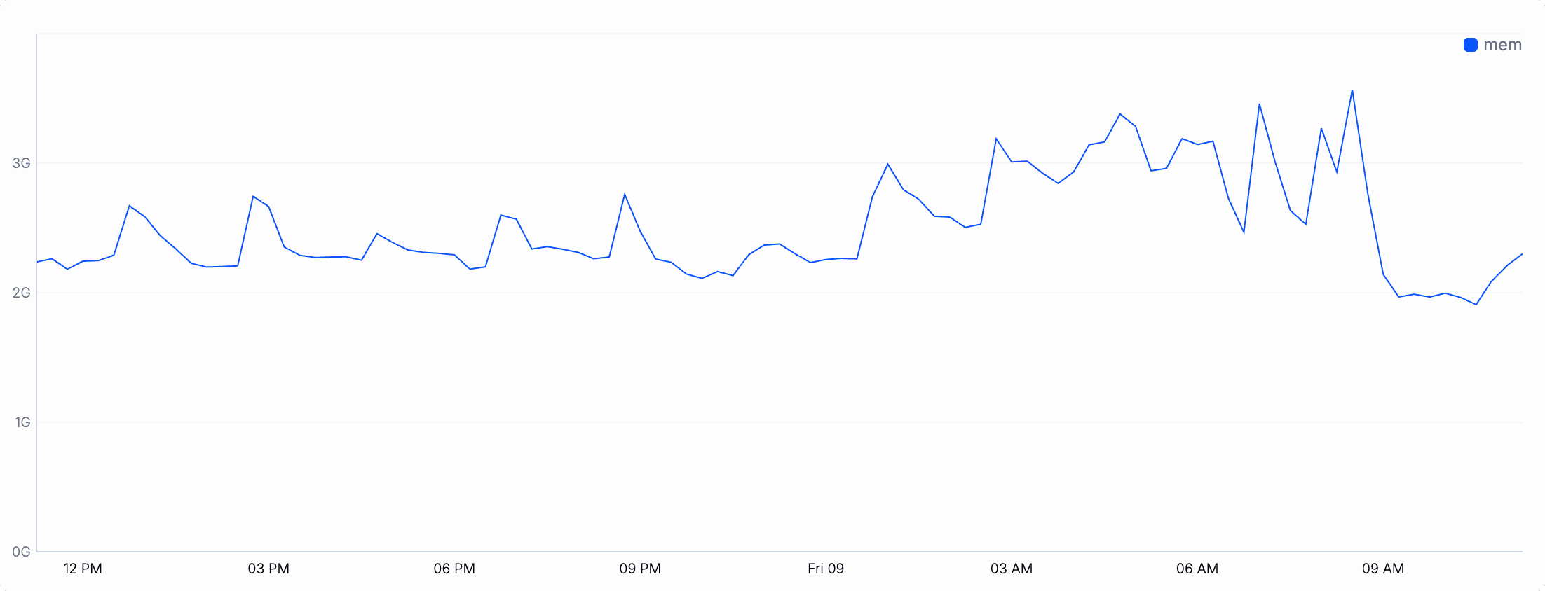

   

   This looks a lot smoother! Pro tip: you can even further optimize the above pipeline by using additional operator arguments.

Compare multiple series

Our metrics data not only includes the current memory usage but also peak usage. Comparing the these two in the same chart helps us understand potentially dangerous spikes. Let's add that second series to the y-axis by upgrading from a single value to a record that represents the series.

metrics "process"
where timestamp > now() - 1d
chart_line (
  x=timestamp,
  y={current: mean(current_memory_usage), peak: max(peak_memory_usage * 1Ki)},
  resolution=15min
)

Because current_memory_usage comes in gigabytes and peak_memory_usage in megabytes, we cannot compare them directly. Hence we normalized the peak usage to gigabytes to make them comparable in a single plot.

If you cannot enumerate the series to plot statically in a record, use the group option to specify a field that contains a unique identifier per series. Here's an example that plots the number of events per pipeline:

metrics "publish"
chart_line (
  x=timestamp,
  y=sum(events),
  x_min=now()-1d,
  group=pipeline_id,
  resolution=30min,
)

Plot distributions as area chart

Area charts are fantastic for visualizing quantities that accumulate over a continuous variable, such as time or value ranges. They are similar to line charts but emphasize the volume underneath the line.

In the above section about line charts, you can exchange every call to chart_line with chart_area and will get a working plot.

from (
  {time: 1, a: 10, b: 20},
  {time: 2, a: 8, b: 25},
  {time: 3, a: 14, b: 30},
  {time: 4, a: 10, b: 25},
  {time: 5, a: 18, b: 40},
)
chart_area x=time, y={a: a, b: b}

The area under the curve gives you a strong visual impression of the total event volume over time.

Stack multiple series

Like bar charts, area charts can display stacked series. This means that the values of the series add up, helping you compare contributions from different groups while still highlighting the overall cumulative shape.

Pass position="stacked" to see the difference:

from (
  {time: 1, a: 10, b: 20},
  {time: 2, a: 8, b: 25},
  {time: 3, a: 14, b: 30},
  {time: 4, a: 10, b: 25},
  {time: 5, a: 18, b: 40},
)
chart_area x=time, y={a: a, b: b}, position="stacked"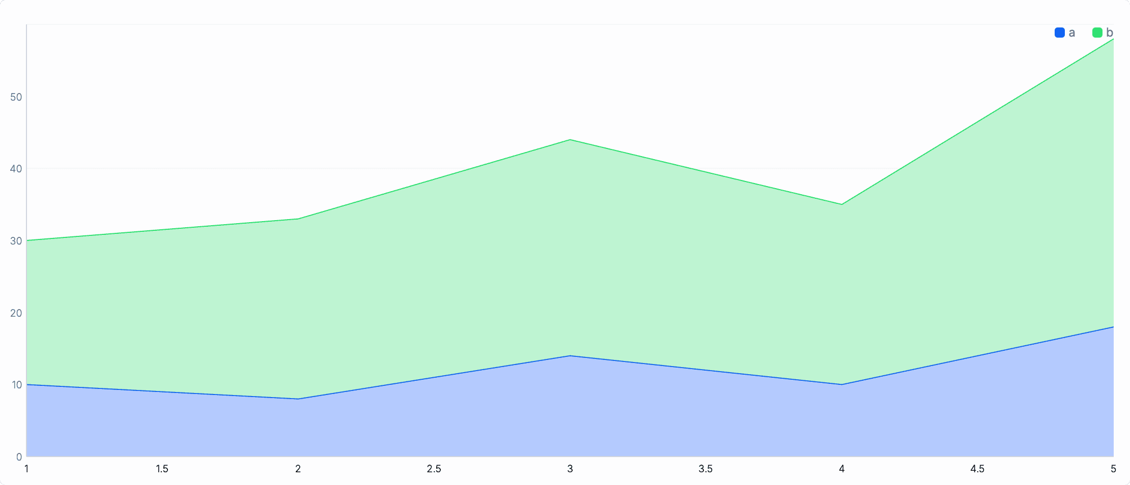

Notice the difference in the y-axis interpretation:

• Without stacking, the areas overlap each other.
• With stacking, the areas become disjoint and cumulatively add up to the total height.

Optimize Plotting with Inline Expressions

While it's intuitive to first prepare your data and then start thinking about how to parameterize your chart operator, this leaves some opportunities for optimization and better results on the table. That's why the chart_* operators offer additional options for inline filtering, rounding, and summarization. These options allow you often to immediately jump to charting without having to think too much about data prepping.

To appreciate these optimization, let's start with our metrics pipeline from the above line chart example:

metrics "process"
where timestamp > now() - 1d                         // filtering
set timestamp = timestamp.round(15min)               // rounding
summarize timestamp, mem=mean(current_memory_usage)  // aggregation
chart_line x=timestamp, y=mem

You can push the filtering, rounding, and aggregation into the chart operator:

metrics "process"
chart_line (
  x=timestamp,
  y=mean(current_memory_usage), // aggregation
  resolution=15min,             // rounding (= flooring)
  x_min=now() - 1d,             // filtering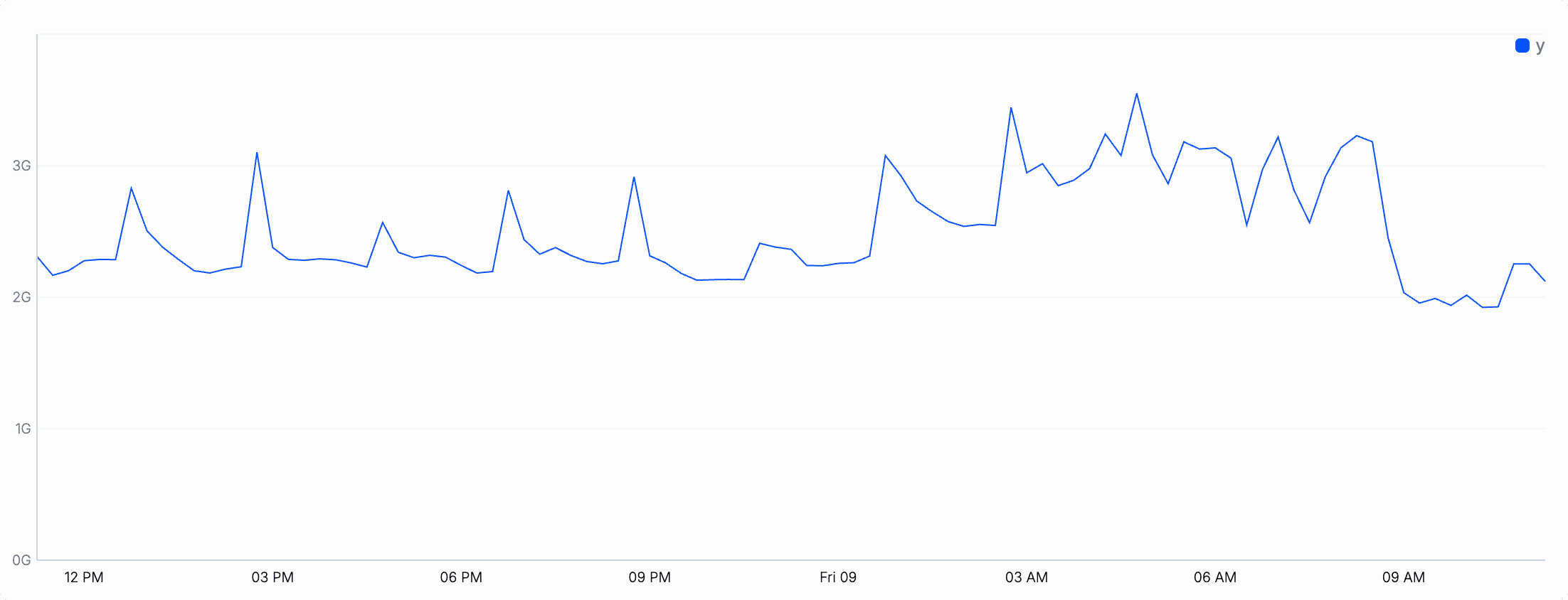
)

Note how this make the pipeline more succinct by removing the extra where, set, and summarize operators.

Here are some important details to remember:

• The x_min/x_max (also y_min/y_max) options set the visible axis domain to fixed interval. Use these options to crop or expand the viewport.
• When using the x_min or x_max options, the chart operator implicitly filters your data for the correct time range, just as if you had specified where x >= floor(x_min, resolution) and x < ceil(x_max, resolution). This avoids needing to specify the ranges twice, and makes sure that the resolution is taken into account correctly.
• Specifying a duration with resolution option creates nicer buckets than naïve rounding, as it uses a dynamic floor for the minimum and a ceiling for the maximum value in the respective bucket. This results in nicer axis ticks that align on the bucket boundary, e.g., hourly or daily.
• The combination of resolution with an aggregation function for the y series is equivalent to the manual summarize.
• When you use resolution, you can additionally use the fill option to patch up missing values with a provided value, e.g., fill=0 replaces otherwise empty buckets with a data point in the plot.